Theta function

For other θ functions, see Theta function (disambiguation).

In mathematics, theta functions are special functions of several complex variables. They are important in many areas, including the theories of abelian varieties and moduli spaces, and of quadratic forms. They have also been applied to soliton theory. When generalized to a Grassmann algebra, they also appear in quantum field theory, specifically string theory and D-branes. A theta function is graphed on a polar coordinate system.

The most common form of theta function is that occurring in the theory of elliptic functions. With respect to one of the complex variables (conventionally called z), a theta function has a property expressing its behavior with respect to the addition of a period of the associated elliptic functions, making it a quasiperiodic function. In the abstract theory this comes from a line bundle condition of descent.

1 Jacobi theta function
2 Auxiliary functions
3 Jacobi identities
4 Theta functions in terms of the nome
5 Product representations
6 Integral representations
7 Explicit values
8 Relation to the Riemann zeta function
9 Relation to the Weierstrass elliptic function
10 Some relations to modular forms
11 A solution to heat equation
12 Relation to the Heisenberg group
13 Generalizations
14 Notes
15 References
16 External links

Jacobi theta function

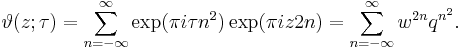
There are several closely related functions called Jacobi theta functions, and many different and incompatible systems of notation for them. One Jacobi theta function (named after Carl Gustav Jacob Jacobi) is a function defined for two complex variables z and τ, where z can be any complex number and τ is confined to the upper half-plane, which means it has positive imaginary part. It is given by the formula

$\vartheta(z; \tau) = \sum_{n=-\infty}^\infty \exp (\pi i n^2 \tau %2B 2 \pi i n z) = 1 %2B 2 \sum_{n=1}^\infty \left(e^{\pi i\tau}\right)^{n^2} \cos(2\pi n z) = \sum_{n=-\infty}^\infty q^{n^2}\zeta^n$

where q = exp(πiτ) and ζ = exp(2πiz). It is a Jacobi form. If τ is fixed, this becomes a Fourier series for a periodic entire function of z with period 1; in this case, the theta function satisfies the identity

$\vartheta(z%2B1; \tau) = \vartheta(z; \tau).$

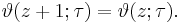
The function also behaves very regularly with respect to its quasi-period τ and satisfies the functional equation

$\vartheta(z%2Ba%2Bb\tau;\tau) = \exp(-\pi i b^2 \tau -2 \pi i b z)\,\vartheta(z;\tau)$

where a and b are integers.

Auxiliary functions

The Jacobi theta function defined above is sometimes considered along with three auxiliary theta functions, in which case it is written with a double 0 subscript:

$\vartheta_{00}(z;\tau) = \vartheta(z;\tau)$

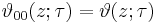
The auxiliary (or half-period) functions are defined by

$\begin{align} \vartheta_{01}(z;\tau)& = \vartheta\!\left(z%2B{\textstyle\frac{1}{2}};\tau\right)\\[3pt] \vartheta_{10}(z;\tau)& = \exp\!\left({\textstyle\frac{1}{4}}\pi i \tau %2B \pi i z\right) \vartheta\!\left(z %2B {\textstyle\frac{1}{2}}\tau;\tau\right)\\[3pt] \vartheta_{11}(z;\tau)& = \exp\!\left({\textstyle\frac{1}{4}}\pi i \tau %2B \pi i\!\left(z%2B{\textstyle \frac{1}{2}}\right)\right)\vartheta\!\left(z%2B{\textstyle\frac{1}{2}}\tau %2B {\textstyle\frac{1}{2}};\tau\right). \end{align}$

This notation follows Riemann and Mumford; Jacobi's original formulation was in terms of the nome q = exp(πiτ) rather than τ. In Jacobi's notation the θ-functions are written like this:

$\begin{align} \theta_1(z;q) &= -\vartheta_{11}(z;\tau)\\ \theta_2(z;q) &= \vartheta_{10}(z;\tau)\\ \theta_3(z;q) &= \vartheta_{00}(z;\tau)\\ \theta_4(z;q) &= \vartheta_{01}(z;\tau) \end{align}$

The above definitions of the Jacobi theta functions are by no means unique. See Jacobi theta functions - notational variations for further discussion.

If we set z = 0 in the above theta functions, we obtain four functions of τ only, defined on the upper half-plane (sometimes called theta constants.) These can be used to define a variety of modular forms, and to parametrize certain curves; in particular, the Jacobi identity is

$\vartheta_{00}(0;\tau)^4 = \vartheta_{01}(0;\tau)^4 %2B \vartheta_{10}(0;\tau)^4$

which is the Fermat curve of degree four.

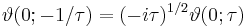
Jacobi identities

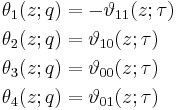
Jacobi's identities describe how theta functions transform under the modular group, which is generated by τ ↦ τ+1 and τ ↦ -1/τ. We already have equations for the first transformation; for the second, let

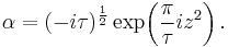
$\alpha = (-i \tau)^{\frac{1}{2}} \exp\!\left(\frac{\pi}{\tau} i z^2 \right).\,$

Then

$\begin{align} \vartheta_{00}\!\left({\textstyle\frac{z}{\tau}; \frac{-1}{\tau}}\right)& = \alpha\,\vartheta_{00}(z; \tau)\quad& \vartheta_{01}\!\left({\textstyle\frac{z}{\tau}; \frac{-1}{\tau}}\right)& = \alpha\,\vartheta_{10}(z; \tau)\\[3pt] \vartheta_{10}\!\left({\textstyle\frac{z}{\tau}; \frac{-1}{\tau}}\right)& = \alpha\,\vartheta_{01}(z; \tau)\quad& \vartheta_{11}\!\left({\textstyle\frac{z}{\tau}; \frac{-1}{\tau}}\right)& = -i\alpha\,\vartheta_{11}(z; \tau). \end{align}$

Theta functions in terms of the nome

Instead of expressing the Theta functions in terms of $z\,$ and $\tau \,$ , we may express them in terms of arguments $w\,$ and the nome q, where $w=e^{\pi {\mathrm{i}}z}\,$ and $q=e^{\pi {\mathrm{i}}\tau}\,$ . In this form, the functions become

$\begin{align} \vartheta_{00}(w, q)& = \sum_{n=-\infty}^\infty (w^2)^n q^{n^2}\quad& \vartheta_{01}(w, q)& = \sum_{n=-\infty}^\infty (-1)^n (w^2)^n q^{n^2}\\[3pt] \vartheta_{10}(w, q)& = \sum_{n=-\infty}^\infty (w^2)^{\left(n%2B1/2\right)} q^{\left(n %2B 1/2\right)^2}\quad& \vartheta_{11}(w, q)& = i \sum_{n=-\infty}^\infty (-1)^n (w^2)^{\left(n%2B1/2\right)} q^{\left(n %2B 1/2\right)^2}. \end{align}$

We see that the Theta functions can also be defined in terms of w and q, without a direct reference to the exponential function. These formulas can, therefore, be used to define the Theta functions over other fields where the exponential function might not be everywhere defined, such as fields of p-adic numbers.

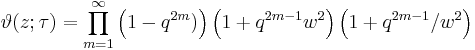
Product representations

The Jacobi triple product tells us that for complex numbers w and q with |q| < 1 and w ≠ 0 we have

$\prod_{m=1}^\infty \left( 1 - q^{2m}\right) \left( 1 %2B w^{2}q^{2m-1}\right) \left( 1 %2B w^{-2}q^{2m-1}\right) = \sum_{n=-\infty}^\infty w^{2n}q^{n^2}.$

It can be proven by elementary means, as for instance in Hardy and Wright's An Introduction to the Theory of Numbers.

If we express the theta function in terms of the nome $q = \exp(\pi i \tau)$ and $w = \exp(\pi i z)$ then

$\vartheta(z; \tau) = \sum_{n=-\infty}^\infty \exp(\pi i \tau n^2) \exp(\pi i z 2n) = \sum_{n=-\infty}^\infty w^{2n}q^{n^2}.$

We therefore obtain a product formula for the theta function in the form

$\vartheta(z; \tau) = \prod_{m=1}^\infty \left( 1 - \exp(2m \pi i \tau)\right) \left( 1 %2B \exp((2m-1) \pi i \tau %2B 2 \pi i z)\right) \left( 1 %2B \exp((2m-1) \pi i \tau -2 \pi i z)\right).$

In terms of w and q:

$\vartheta(z; \tau) = \prod_{m=1}^\infty \left( 1 - q^{2m})\right) \left( 1 %2B q^{2m-1}w^2\right) \left( 1 %2B q^{2m-1}/w^2\right)$

$= (q^2;q^2)_\infty\,(-w^2q;q^2)_\infty\,(-q/w^2;q^2)_\infty$

$= (q^2;q^2)_\infty\,\theta(-w^2q;q^2)$

where $(\cdot \cdot)_\infty$ is the q-Pochhammer symbol and $\theta(\cdot \cdot)$ is the q-theta function. Expanding terms out, the Jacobi triple product can also be written

$\prod_{m=1}^\infty \left( 1 - q^{2m}\right) \left( 1 %2B (w^{2}%2Bw^{-2})q^{2m-1}%2Bq^{4m-2}\right),$

which we may also write as

$\vartheta(z|q) = \prod_{m=1}^\infty \left( 1 - q^{2m}\right) \left( 1 %2B 2 \cos(2 \pi z)q^{2m-1}%2Bq^{4m-2}\right).$

This form is valid in general but clearly is of particular interest when z is real. Similar product formulas for the auxiliary theta functions are

$\vartheta_{01}(z|q) = \prod_{m=1}^\infty \left( 1 - q^{2m}\right) \left( 1 - 2 \cos(2 \pi z)q^{2m-1}%2Bq^{4m-2}\right).$

$\vartheta_{10}(z|q) = 2 q^{1/4}\cos(\pi z)\prod_{m=1}^\infty \left( 1 - q^{2m}\right) \left( 1 %2B 2 \cos(2 \pi z)q^{2m}%2Bq^{4m}\right).$

$\vartheta_{11}(z|q) = -2 q^{1/4}\sin(\pi z)\prod_{m=1}^\infty \left( 1 - q^{2m}\right) \left( 1 - 2 \cos(2 \pi z)q^{2m}%2Bq^{4m}\right).$

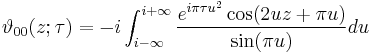
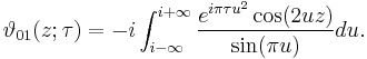
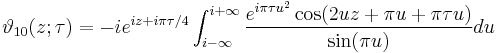
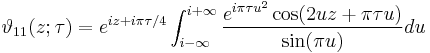
Integral representations

The Jacobi theta functions have the following integral representations:

$\vartheta_{00} (z; \tau) = -i \int_{i - \infty}^{i %2B \infty} {e^{i \pi \tau u^2} \cos (2 u z %2B \pi u) \over \sin (\pi u)} du$

$\vartheta_{01} (z; \tau) = -i \int_{i - \infty}^{i %2B \infty} {e^{i \pi \tau u^2} \cos (2 u z) \over \sin (\pi u)} du.$

$\vartheta_{10} (z; \tau) = -i e^{iz %2B i \pi \tau / 4} \int_{i - \infty}^{i %2B \infty} {e^{i \pi \tau u^2} \cos (2 u z %2B \pi u %2B \pi \tau u) \over \sin (\pi u)} du$

$\vartheta_{11} (z; \tau) = e^{iz %2B i \pi \tau / 4} \int_{i - \infty}^{i %2B \infty} {e^{i \pi \tau u^2} \cos (2 u z %2B \pi \tau u) \over \sin (\pi u)} du$

Explicit values

See ^[1]

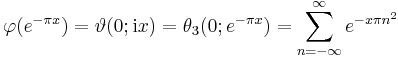
$\varphi(e^{-\pi x}) = \vartheta(0; {\mathrm{i}}x) = \theta_3(0;e^{-\pi x}) = \sum_{n=-\infty}^\infty e^{-x \pi n^2}$

$\varphi\left(e^{-\pi} \right) = \frac{\sqrt[4]{\pi}}{\Gamma(\frac{3}{4})}$

$\varphi\left(e^{-2\pi} \right) = \frac{\sqrt[4]{6\pi%2B4\sqrt2\pi}}{2\Gamma(\frac{3}{4})}$

$\varphi\left(e^{-3\pi}\right) = \frac{\sqrt[4]{27\pi%2B18\sqrt3\pi}}{3\Gamma(\frac{3}{4})}$

$\varphi\left(e^{-4\pi}\right) =\frac{\sqrt[4]{8\pi}%2B2\sqrt[4]{\pi}}{4\Gamma(\frac{3}{4})}$

$\varphi\left(e^{-5\pi} \right) =\frac{\sqrt[4]{225\pi%2B 100\sqrt5 \pi}}{5\Gamma(\frac{3}{4})}$

$\varphi\left(e^{-6\pi}\right) = \frac{\sqrt[3]{3\sqrt{2}%2B3\sqrt[4]{3}%2B2\sqrt{3}-\sqrt[4]{27}%2B\sqrt[4]{1728}-4}\cdot \sqrt[8]{243{\pi}^2}}{6\sqrt[6]{1%2B\sqrt6-\sqrt2-\sqrt3}{\Gamma(\frac{3}{4})}}$

Relation to the Riemann zeta function

The relation

$\vartheta(0;-1/\tau)=(-i\tau)^{1/2} \vartheta(0;\tau)$

was used by Riemann to prove the functional equation for the Riemann zeta function, by means of the integral

$\Gamma\left(\frac{s}{2}\right) \pi^{-s/2} \zeta(s) = \frac{1}{2}\int_0^\infty\left[\vartheta(0;it)-1\right] t^{s/2}\frac{dt}{t}$

which can be shown to be invariant under substitution of s by 1 − s. The corresponding integral for z not zero is given in the article on the Hurwitz zeta function.

Relation to the Weierstrass elliptic function

The theta function was used by Jacobi to construct (in a form adapted to easy calculation) his elliptic functions as the quotients of the above four theta functions, and could have been used by him to construct Weierstrass's elliptic functions also, since

$\wp(z;\tau) = -(\log \vartheta_{11}(z;\tau))'' %2B c$

where the second derivative is with respect to z and the constant c is defined so that the Laurent expansion of $\wp(z)$ at z = 0 has zero constant term.

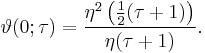
Some relations to modular forms

Let η be the Dedekind eta function. Then

$\vartheta(0;\tau)=\frac{\eta^2\left(\tfrac{1}{2}(\tau%2B1)\right)}{\eta(\tau%2B1)}.$

A solution to heat equation

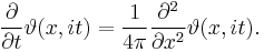
The Jacobi theta function is the unique solution to the one-dimensional heat equation with periodic boundary conditions at time zero. This is most easily seen by taking z = x to be real, and taking τ = it with t real and positive. Then we can write

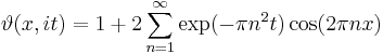
$\vartheta (x,it)=1%2B2\sum_{n=1}^\infty \exp(-\pi n^2 t) \cos(2\pi nx)$

which solves the heat equation

$\frac{\partial}{\partial t} \vartheta(x,it)=\frac{1}{4\pi} \frac{\partial^2}{\partial x^2} \vartheta(x,it).$

That this solution is unique can be seen by noting that at t = 0, the theta function becomes the Dirac comb:

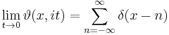
$\lim_{t\rightarrow 0} \vartheta(x,it)=\sum_{n=-\infty}^\infty \delta(x-n)$

where δ is the Dirac delta function. Thus, general solutions can be specified by convolving the (periodic) boundary condition at t = 0 with the theta function.

Relation to the Heisenberg group

The Jacobi theta function is invariant under the action of a discrete subgroup of the Heisenberg group. This invariance is presented in the article on the theta representation of the Heisenberg group.

Generalizations

If F is a quadratic form in n variables, then the theta function associated with F is

$\theta_F (z)= \sum_{m\in Z^n} \exp(2\pi izF(m))$

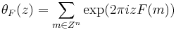
with the sum extending over the lattice of integers Zⁿ. This theta function is a modular form of weight n/2 (on an appropriately defined subgroup) of the modular group. In the Fourier expansion,

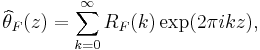
$\widehat{\theta}_F (z) = \sum_{k=0}^\infty R_F(k) \exp(2\pi ikz),$

the numbers R_F(k) are called the representation numbers of the form.

Ramanujan theta function

Further information: Ramanujan theta function and mock theta function

Riemann theta function

Let

$\mathbb{H}_n=\{F\in M(n,\mathbb{C}) \; \mathrm{s.t.}\, F=F^T \;\textrm{and}\; \mbox{Im} F >0 \}$

be set of symmetric square matrices whose imaginary part is positive definite. H_n is called the Siegel upper half-space and is the multi-dimensional analog of the upper half-plane. The n-dimensional analogue of the modular group is the symplectic group Sp(2n,Z); for n = 1, Sp(2,Z) = SL(2,Z). The n-dimensional analog of the congruence subgroups is played by $\textrm{Ker} \{\textrm{Sp}(2n,\mathbb{Z})\rightarrow \textrm{Sp}(2n,\mathbb{Z}/k\mathbb{Z}) \}$ .

Then, given $\tau\in \mathbb{H}_n$ , the Riemann theta function is defined as

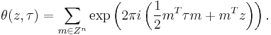
$\theta (z,\tau)=\sum_{m\in Z^n} \exp\left(2\pi i \left(\frac{1}{2} m^T \tau m %2Bm^T z \right)\right).$

Here, $z\in \mathbb{C}^n$ is an n-dimensional complex vector, and the superscript T denotes the transpose. The Jacobi theta function is then a special case, with n = 1 and $\tau \in \mathbb{H}$ where $\mathbb{H}$ is the upper half-plane.

The Riemann theta converges absolutely and uniformly on compact subsets of $\mathbb{C}^n\times \mathbb{H}_n.$

The functional equation is

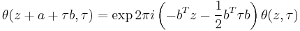
$\theta (z%2Ba%2B\tau b, \tau) = \exp 2\pi i \left(-b^Tz-\frac{1}{2}b^T\tau b\right) \theta (z,\tau)$

which holds for all vectors $a,b \in \mathbb{Z}^n$ , and for all $z \in \mathbb{C}^n$ and $\tau \in \mathbb{H}_n$ .

Poincaré series

The Poincaré series generalizes the theta series to automorphic forms with respect to arbitrary Fuchsian groups.

Notes

^ Jinhee, Yi (2004), "Theta-function identities and the explicit formulas for theta-function and their applications", Journal of Mathematical Analysis and Applications 292: 381–400, doi:10.1016/j.jmaa.2003.12.0091.

References

Abramowitz, Milton & Stegun, Irene A. (1964), Handbook of Mathematical Functions, New York: Dover Publications, ISBN 0486612724 . (See section 16.27ff.)
Akhiezer, Naum Illyich (1990) [1970], Elements of the Theory of Elliptic Functions, AMS Translations of Mathematical Monographs, 79, Providence, RI: AMS, ISBN 0821845322 .
Farkas, Hershel M. & Kra, Irwin (1980), Riemann Surfaces, New York: Springer-Verlag, ISBN 0387904654 . (See Chapter 6 for treatment of the Riemann theta)
Hardy, G. H. & Wright, E. M. (1959), An Introduction to the Theory of Numbers (Fourth ed.), Oxford: Clarendon Press .
Mumford, David (1983), Tata Lectures on Theta I, Boston: Birkhauser, ISBN 3764331097 .
Pierpont, James (1959), Functions of a Complex Variable, New York: Dover .
Rauch, Harry E. & Farkas, Hershel M. (1974), Theta Functions with Applications to Riemann Surfaces, Baltimore: Williams & Wilkins, ISBN 0683071963 .
Reinhardt, William P.; Walker, Peter L. (2010), "Theta Functions", in Olver, Frank W. J.; Lozier, Daniel M.; Boisvert, Ronald F. et al., NIST Handbook of Mathematical Functions, Cambridge University Press, ISBN 978-0521192255, MR 2723248, http://dlmf.nist.gov/20
Whittaker, E. T. & Watson, G. N. (1927), A Course in Modern Analysis (Fourth ed.), Cambridge: Cambridge University Press . (See chapter XXI for the history of Jacobi's θ functions)

External links

Matlab code for theta function evaluation by elliptic project

This article incorporates material from Integral representations of Jacobi theta functions on PlanetMath, which is licensed under the Creative Commons Attribution/Share-Alike License.